The Binomial Model

Table of Contents

Options Desk Primer - This article is part of a series.

Part 1: This Article

Background
#

This series covers the material an options desk trader (rather than a quant) must know. It consists of seven notes as follows:


1	The Binomial Model	where a fair price comes from
2	The Continuous Limit	the same argument refined into a formula
3	On Risk Sensitivities	what has to be managed once the trade is on
4	Ideal vs. Reality	where the model’s assumptions fail, and what that costs
5	The Volatility Surface	what the market quotes instead of one volatility
6	Risk Under a Surface	what has to be managed once the surface moves
7	Across Asset Classes	what carries to currencies, commodities and rates

Notes 1 to 6 depend on the one before it, while note 7 stands apart and can be read at any point after note 5. The first two notes are one argument split in half at the point where the binomial tree’s backward induction becomes the Black-Scholes PDE; together they are the pricing note. The running example throughout is an equity index, which is a choice rather than a neutral default.¹

Prerequisites

This note assumes the vocabulary but not the theory. Before continuing, you should be able to answer the following questions:

What is the difference between an option and a forward or futures contract?
What is a call, a put, a European option, an American option? What are the intrinsic and time value of an option?
What does it mean to say a stock has a volatility of twenty per cent?
What is a discount factor, and why is a payoff in the future worth less than the same payoff today?

How to Read This Note

The spine is three steps: replicate the payoff with a portfolio of stock and bond, read off the cost of that portfolio as the price, and repeat the same argument at every node of the tree. Everything else explains or builds on those three steps.

Skip on a first read the appendix on the fundamental theorems, which is general theory rather than desk material, and the collapsed note on non-monotone convergence.

If you read only one thing, read When Replication Fails. It is the reason volatility is traded at all.

Pricing by Replication
#

The One-Period Model
#

A pricing model does not predict the future price of a security. It computes the cost of reproducing its payoff in every state of the world, and takes that cost as the fair price. Any other price admits arbitrage.²

The smallest setting in which this can be carried out has one period, two states, and two traded assets: a stochastic stock and a deterministic bond. Over the period the stock moves from $S$ to either $uS$ or $dS$, with $u \gt d$ fixed and known in advance³; the bond earns the risk-free rate $R = e^{r\Delta t}$, where $\Delta t$ is the length of the period. We wish to price a third instrument, an option paying $C_u$ in the up state and $C_d$ in the down state.

We hold $y$ shares and $x$ in the bond, and require the portfolio to match the option in both states:

$$\tag{1.1} \begin{cases} y\,uS + xR = C_u \\ y\,dS + xR = C_d \end{cases}$$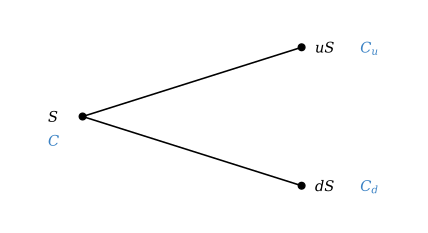

Figure 1.1. The one-period model. The option pays Cu in the up state and Cd in the down state, and is replicated by a portfolio of stock and bond.

Proposition 1A. The system (1.1) has the unique solution

$$\tag{1.2} y = \frac{C_u - C_d}{(u-d)S}, \qquad x = \frac{1}{R}\left(C_u - y\,uS\right),$$

and since this portfolio pays what the option pays, the option is worth $C = yS + x$.

The quantity $y$ is a hedge ratio: the number of shares that makes the position insensitive to which state occurs, determined by solving the system (1.1).

Note that (1.1) contains no probabilities: the likelihood of an up move is absent from the construction, so it is absent from the price. Two traders who disagree about the stock’s prospects but agree on $u$ and $d$ must quote the same option.

Risk-Neutral Probabilities
#

Substituting (1.2) into $C = yS + x$ and collecting terms yields a second form of the price.

Proposition 1B. The option price may be written

$$\tag{1.3} C = \frac{1}{R}\left[q\,C_u + (1-q)\,C_d\right], \qquad q = \frac{R-d}{u-d}.$$

The right side of (1.3) is a weighted average of the two payoffs, discounted at the risk-free rate. The weights sum to one by construction. If they are also positive, they satisfy the requirements of a probability distribution over the two states, and (1.3) may be read as a discounted expectation, although no expectation was taken in deriving it.

This is the origin of probabilistic language in derivative pricing. It is a reinterpretation of an algebraic identity, adopted because expectations generalize more easily than systems of replication equations. The weights are called risk-neutral probabilities, and they are not anyone’s forecast.

Whether the weights qualify as probabilities is a genuine condition.

Proposition 1C. $0 \lt q \lt 1$ if and only if $d \lt R \lt u$.

The condition $d \lt R \lt u$ is exactly the absence of arbitrage.⁴ Absence of arbitrage and admissibility of the probabilistic reading are therefore the same statement.⁵

On the Name “Risk-Neutral”

The term suggests an assumption about investor preferences. No such assumption enters the derivation of (1.3). Under the risk-neutral weights the underlying grows at the risk-free rate, but that is a property of the numbers we constructed, not a description of anyone’s expectations.

When Replication Fails
#

Everything above worked because the market had two instruments and two states. Add a third state and it stops working, and what breaks is worth seeing because it is the situation a desk is actually in.

Suppose the stock can move to $uS$, $mS$, or $dS$. Then failure appears in the replication language: generally no replicating portfolio exists, because three payoffs must be matched with only two instruments. The same failure appears in the probabilistic language of (1.3), where the price is a discounted expectation under risk-neutral weights. Those weights are not pinned down: with three states they must satisfy only two constraints, so a whole family of weights is consistent with the market, each giving a different option price. The positive members of that family are the arbitrage-free ones, by Proposition 1C,⁶ and what replaces a single price is a bounded interval of prices.⁷

A market in which every payoff can be replicated is called complete. The two-state model is complete only because it happens to have as many instruments as states. Completeness in the replication language means replication always works; completeness in the probabilistic language means the risk-neutral weights are unique. These are not two facts: they are one fact stated in two languages.

The reason this matters is that the third state is not a hypothetical. Any second source of risk plays the same role as that third state, and the most important one is volatility itself. Once volatility can move, stock and bond no longer span the outcomes, so replication fails in the replication language and the weights are not unique in the probabilistic language. Thus the price is genuinely not unique. Every model that admits random volatility inherits this, which is why the fifth note’s stochastic volatility models come with an admission attached, and why a desk hedges an option with another option rather than with stock alone.

Interview Checkpoint

Questions are tagged concept (definitions, key facts, and common misunderstandings), derivation (reproduce or extend an argument), and application (use a result in a concrete setting). A question may carry more than one tag when it spans categories.

(derivation) Derive $q$ from the one-period replication argument. At which step could the real-world probability have entered?
(application) Two traders disagree on the direction of a stock. Do they disagree on the price of a call? On the profit from holding one?
(derivation) Show that $0 \lt q \lt 1$ is equivalent to the absence of arbitrage. What trade is available if $R \gt u$?
(concept) What is assumed when the weights in (1.3) are called probabilities, and what is not assumed?
(application) Under a model in which volatility is itself random, is the option price unique? Relate the answer to the three-state case.
(application) Price a forward contract by replication. Why is no distributional assumption required?
(derivation) Derive put-call parity by arbitrage. Which assumptions are used? Does it hold for American options?
(concept/derivation) Give the model-free bounds on a European call. Why is $C \geq S_0 - Ke^{-rT}$?
(derivation) Show that an American call on a non-dividend-paying stock is never optimally exercised early. Why does the argument fail for a put, and for a dividend-paying stock?
(concept) A colleague states that risk-neutral pricing assumes investors are indifferent to risk. Correct him.

Answers

Match the option’s payoff in both states with $y$ shares and $x$ in the bond, solve the two equations, and substitute back into $C = yS + x$; collecting terms gives (1.3). The real-world probability could only have entered by weighting the two states, and no step does that: the portfolio is required to match in both states, not on average.
They agree on the price and disagree on the profit. The price follows from replication, which never references direction. The profit from holding a call depends on where the stock actually goes, which is exactly what they disagree about.
$q = (R-d)/(u-d)$ with $u \gt d$, so $q \gt 0$ requires $R \gt d$ and $q \lt 1$ requires $R \lt u$. If $R \gt u$, the bond beats the stock in every state: short the stock, lend the proceeds, and collect the difference with no risk.
Assumed: that the weights are positive and sum to one, which is exactly $d \lt R \lt u$. Not assumed: that they describe anyone’s beliefs, that investors are risk-neutral, or that the stock is expected to grow at $r$.
Not unique. Random volatility is a second source of risk, so the market has more states than independent instruments, the three-state case. Replication fails, the weights form a family rather than a point, and a range of arbitrage-free prices results. A model selects one by calibration.
Buy the stock and borrow $Ke^{-rT}$; at maturity you hold the stock and owe $K$, which is the forward’s payoff. The cost is $S_0 - Ke^{-rT}$. No distribution is needed because the payoff is linear in $S_T$, so a static holding replicates it, no rebalancing, hence no assumption about how it travels.
A call minus a put, plus $Ke^{-rT}$ in the bond, pays $S_T$ in every state, so $C - P + Ke^{-rT} = S$. It uses only no-arbitrage and European exercise, and no distributional assumption. It fails as an equality for American options, since early exercise breaks the static replication; only an inequality survives.
$\max(0,\ S_0 - Ke^{-rT}) \leq C \leq S_0$. The lower bound holds because the call dominates the forward, which is worth $S_0 - Ke^{-rT}$; if the call were cheaper, buy it, sell the forward, and lock in the difference. The upper bound holds because the stock itself dominates any right to buy it.
Exercising early surrenders the remaining time value and pays $K$ sooner than necessary. Holding the option plus $Ke^{-rT}$ in the bond dominates owning the stock in every state, so exercise is never optimal, and the American call is worth the European. For a put, exercising releases cash that earns interest, which can outweigh the time value. A dividend restores early exercise for calls, since the holder forgoes it by not owning the stock.
The weights are constructed to make the replication identity hold; they are not beliefs. No statement about preferences enters the derivation of (1.3), which is pure algebra on a hedging portfolio. Under $\mathbb{Q}$ the stock does grow at $r$, but that is a property of the numbers we built, not a claim about anyone’s expectations.

From One Period to Multi Period
#

Backward Induction
#

Repeating the one-period construction over successive intervals produces a tree: a grid of nodes, each carrying a stock price, connected by the moves available from it. Taking $d = 1/u$ makes an up move followed by a down move return to the original price, so that the tree recombines.⁸

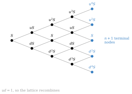
Figure 1.2. A recombining tree over four periods. An up move followed by a down move returns to the starting price.

Pricing proceeds by backward induction. We write the payoff at every terminal node, apply (1.3) at each node of the preceding column, and repeat until reaching the root. Every step is the one-period argument of Proposition 1A, so the tree describes not only the price but the trading strategy that produces it, with (1.2) giving the stock and bond positions to carry out of each node.

Backward induction works because of the Markov property of the stock price: what happens next depends on where the price is now and not on how it arrived. A node therefore carries all the information needed to price from that node onward, and one number per node suffices.⁹

Example: A Two-Period Tree Carried Through

Take $S_0 = 100$, $u = 1.10$, $d = 1/u$, two periods, $r = 0$, and a call struck at 100. Then $R = 1$ and $q = (1-d)/(u-d) = 0.4762$.

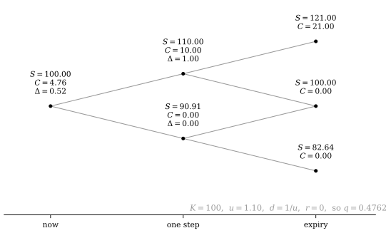
Figure 1.3. The same construction with numbers in it. Each node carries the stock price, the option value, and the shareholding to carry out of it.

Work right to left. At expiry the payoffs are $121 - 100 = 21$, $0$ and $0$. At the upper node of the middle column, (1.3) gives $0.4762 \times 21 = 10.00$; at the lower node both successors pay nothing, so the value is $0$. At the root, $0.4762 \times 10.00 = 4.76$.

The hedge ratios come from (1.2) at the same time. At the root, $y = (10.00-0)/((1.10-0.9091)\times100) = 0.52$ shares. In the upper node it rises to $1.00$ (the option is certain to finish in the money from there, so it is a share) and in the lower node it falls to $0$.

That movement of the hedge ratio from 0.52 toward either 1 or 0 is the whole of what a delta-hedged position does for a living, and it is gamma seen at two-period resolution.

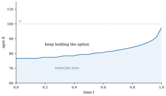
American options require one additional comparison. The holder takes the better of continuing and exercising, so the value at a node is

$$\tag{1.4} C_{\text{node}} = \max\left\{\underbrace{\frac{1}{R}\left[qC_u + (1-q)C_d\right]}_{\text{value of holding}},\quad \text{value of exercising now}\right\}.$$

This is a dynamic-programming problem and admits no closed-form solution, which is the principal reason binomial pricing models remain in use.

The comparison does not always bind. The governing intuition is that exercising early surrenders the remaining time value, so it is only rational when something else compensates, interest earned on the strike, in the case of a put, or a dividend forgone, in the case of a call. An American call on a stock paying no dividend has neither, so it is never exercised early and is worth exactly the European call. The dominance argument behind that claim was question 9 of the previous checkpoint; the full set of cases is set out in the fourth note, alongside the question of how a dividend should be modelled in the first place.

Figure 1.4. The early exercise boundary for an American put. Below the boundary the holder should exercise at once; above it, keeping the option alive is worth more. The boundary rises toward the strike as expiry approaches. An American call on a non-dividend-paying stock has no such boundary.

The Cox-Ross-Rubinstein Parametrization
#

Nothing so far determines $u$ and $d$. Cox, Ross, and Rubinstein choose them so that the variance of the tree matches a volatility $\sigma$ over each interval:

$$\tag{1.5} u = e^{\sigma\sqrt{\Delta t}}, \qquad d = e^{-\sigma\sqrt{\Delta t}} = \frac{1}{u}, \qquad q = \frac{e^{r\Delta t}-d}{u-d}, \qquad \Delta t = \frac{T}{n}.$$

Theorem 1D. Under the parametrization (1.5), the tree price converges to the Black-Scholes-Merton price as $n \to \infty$.

The convergence rests on three observations. First, the log price is additive: $\ln S_T = \ln S_0 + \sum_{i=1}^n X_i$, where each step contributes $X_i = \pm\sigma\sqrt{\Delta t}$, independent and identically distributed. A sum of many such steps becomes normally distributed, by the Central Limit Theorem. So $\ln S_T$ approaches a normal distribution, and $S_T$, being the exponential of it, approaches a lognormal one. Second, each step contributes $\sigma^2\Delta t$ to the variance of the log price, so the total variance is $\sigma^2T$ for every $n$. Third, re-hedging at every node becomes re-hedging continuously.

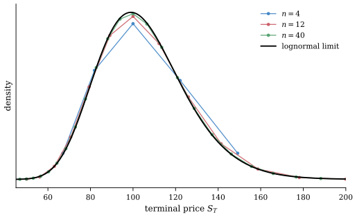
Figure 1.5. The terminal distribution of the tree for increasing numbers of steps, approaching the lognormal density.

The $\sqrt{\Delta t}$ scaling in (1.5) holds the total variance fixed as the grid is refined, and is the reason price moves scale as the square root of time. The third observation is the assumption examined in the fourth note of this series.

Optional: Convergence is Not Monotone

Convergence is of order $1/n$ but oscillatory. The strike generally falls between two terminal nodes, and its relative position shifts with $n$, so refining the grid produces a sawtooth rather than a smooth approach. Increasing $n$ is therefore an unreliable way to obtain accuracy. Practical implementations use Richardson extrapolation, averaging over adjacent $n$, or node placement aligned to the strike.

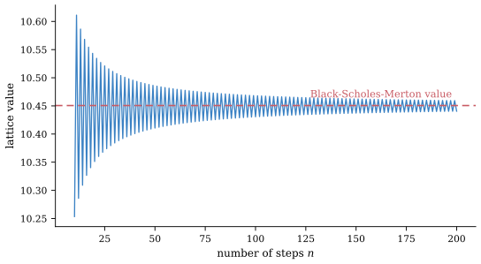
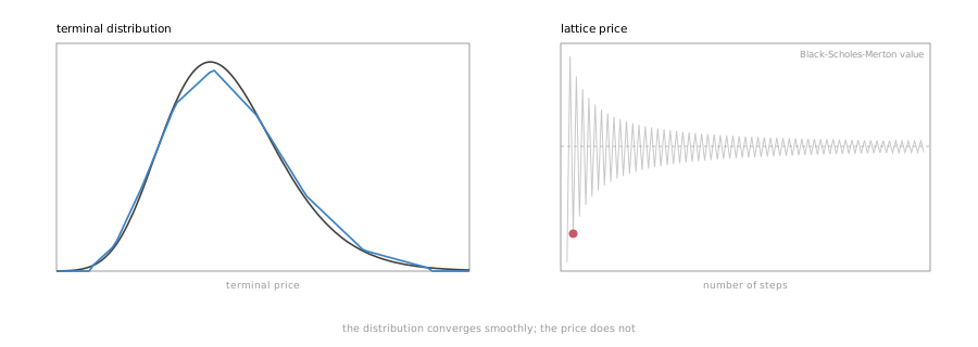
Figure 1.6. Convergence of the tree price to the Black-Scholes-Merton price. The approach is oscillatory rather than monotone.

Figure 1.7. Refining the tree, animated. The terminal distribution settles smoothly onto the lognormal while the price oscillates around the Black-Scholes-Merton value rather than approaching it from one side.

The animation makes the asymmetry plain. The distribution converges the way one would hope, each refinement moving it closer to the lognormal. The price does not: it overshoots and undershoots, and a tree with more steps is not reliably more accurate than one with fewer. This is why the practical advice is to average adjacent $n$ or extrapolate, rather than simply to refine.

Interview Checkpoint

Questions are tagged concept (definitions and key facts), derivation (reproduce or extend an argument), and application (use a result in a concrete setting). A question may carry more than one tag when it spans categories.

(concept) Why choose $d = 1/u$? What is the cost of not doing so?
(application) Price a two-period European call by hand, then the American put on the same tree. Where do the procedures differ?
(derivation) Why must $u$ scale as $e^{\sigma\sqrt{\Delta t}}$ rather than $e^{\sigma\Delta t}$? What limit does the wrong scaling produce?
(concept) Write down the replicating portfolio at a node. How much is borrowed in the bond, and what does it correspond to in the continuous model?
(derivation) Sketch the proof of Theorem 1D. Why is the convergence oscillatory, and why does the terminal distribution not share that behaviour?
(application) How are delta and gamma extracted from a tree? Why are they noisier than closed-form sensitivities?
(concept) What does a trinomial tree provide? Is it more accurate per node, or per unit of computation?
(application) How is a discrete cash dividend incorporated? Why does this break recombination?
(application) Price a knock-out barrier on a tree. Why does accuracy degrade, and what corrects it?
(concept) As $n \to \infty$, what happens to the number of shares traded by the replicating strategy?

Answers

It makes an up move followed by a down move return to the starting price, so the tree recombines and $n$ steps produce $n+1$ terminal nodes rather than $2^n$. Without it the tree is still correct but the node count grows exponentially, which is unusable beyond a few dozen steps.
For the European call, take the payoff at the four terminal nodes and apply (1.3) twice. For the American put, do the same but at every intermediate node take the larger of the discounted expectation and the value of exercising now, per (1.4). The difference is the comparison at each node, the European calculation never looks at intrinsic value before expiry.
Because variance accumulates linearly in time, so the standard deviation of the log price over one step must scale as $\sqrt{\Delta t}$. With $e^{\sigma\Delta t}$ the total variance would vanish as the grid is refined, and the limit would be a deterministic path rather than a diffusion.
$y = (C_u - C_d)/((u-d)S)$ shares and $x = (C_u - y\,uS)/R$ in the bond, which is negative for a long call; you borrow. That borrowing is the financing term $r(C - S\Delta)$ in the continuous PDE (2.1).
The log price is a sum of i.i.d. steps, so the Central Limit Theorem makes it normal in the limit and $S_T$ lognormal; each step contributes $\sigma^2\Delta t$ of variance, so total variance is $\sigma^2T$ for every $n$. The price oscillates because the strike generally lies between two terminal nodes and its relative position shifts as $n$ changes. The distribution has no strike, so nothing shifts relative to it and it converges monotonically, which is the contrast Figure 1.7 animates.
By finite differences on the tree: delta from adjacent nodes at the first step, gamma from three nodes at the second. They are noisier because the node spacing is coarse and its position relative to the strike moves with $n$, so the same oscillation that affects the price affects its differences more strongly.
A middle branch, which places nodes at the strike and improves stability for barriers and for Greeks. It is more accurate per node but not necessarily per unit of computation, since each node costs more.
Subtract the dividend from the stock price at the ex-date node. This breaks recombination because a proportional up-then-down move no longer returns to the same price once a fixed cash amount has been removed, so the node count stops growing linearly. The standard remedy, and the wider consequences of modelling a discrete dividend as a smooth yield, are taken up in the fourth note.
Price it by backward induction, setting the value to zero at any node beyond the barrier. Accuracy degrades badly because the barrier generally falls between node levels, so the tree effectively monitors a barrier displaced from the true one. The fix is to align the grid so a layer of nodes sits exactly on the barrier.
It grows without bound. The strategy rebalances at every node, and the total quantity traded diverges as the grid is refined, which is exactly why frictions, treated in the fourth note, make continuous hedging impossible in practice.

Common Mistakes

“Risk-neutral pricing assumes investors don’t care about risk.” No preference assumption enters anywhere. The weights are constructed so that the replication identity holds; that they can be read as probabilities is a consequence of no-arbitrage, not an input.

“The real probability of an up move must matter somewhere.” It cannot. The portfolio is required to match the payoff in both states, not on average, so nothing in the construction can weight one state against the other.

“A tree with more steps is more accurate.” Not reliably. Convergence is oscillatory, because the strike sits between terminal nodes and its relative position shifts with $n$. Averaging the prices from adjacent values of $n$ beats increasing $n$ further.

“Recombination is just an efficiency trick.” It is, but the efficiency is the difference between $n+1$ and $2^n$ terminal nodes, which is the difference between a usable method and an unusable one.

The Minimum Viable Version

If the rest of this note fades, these should not.

A price is a manufacturing cost. It is what reproducing the payoff costs, not a forecast of anything.
The hedge ratio comes first. $y = (C_u - C_d)/((u-d)S)$ is the shareholding that makes the next move irrelevant; the price then follows as the cost of the replicating portfolio.
Probabilities never entered. Two traders who disagree about direction must quote the same option, because (1.1) matches the payoff in both states rather than on average.
Risk-neutral weights are algebra, not beliefs. They exist exactly when $d \lt R \lt u$, which is exactly no-arbitrage.
Replication fails when states outnumber instruments. Then there is a range of arbitrage-free prices, not a price.
Volatility is the second state. Once it can move, stock and bond no longer span the outcomes: this is why options are hedged with options.
A tree is the one-period argument repeated. Backward induction works because the stock is Markov; every node carries a price and a shareholding.
Early exercise needs a reason. Surrendering time value is only rational when interest on the strike or a forgone dividend pays for it.

Appendix: The General Statements (optional)
#

This appendix is optional and not needed for trading. It gives the general form of the two standard results behind the two-state argument.

The counting argument. With $n$ states, a payoff is a vector in $n$-dimensional space. Suppose there are $m$ independent tradable instruments. The payoffs that can be built span a subspace of dimension $m$. The weight vectors consistent with the market are the solution set of the constraints “price every tradable instrument correctly”, of dimension $n-m$. The two dimensions sum to $n$, because they are the same system of equations read in opposite directions.¹⁰ Every extra dimension of payoffs that can be replicated is one fewer dimension of freedom in the weights, exactly.

	replicable payoffs	admissible weights¹¹
two states, a bond and a stock	dimension 2 (everything replicable)	dimension 0 ($q$ unique)
three states, a bond and a stock	dimension 2 (a plane, most payoffs unreachable)	dimension 1 (a family of $q$)
$n$ states, $m$ independent instruments	dimension $m$	dimension $n-m$

The two theorems. Both are stated in terms of a measure $\mathbb{Q}$ assigning weights to future outcomes, playing the role of $q$ above.

First Fundamental Theorem of Asset Pricing. A market admits no arbitrage iff there exists a measure $\mathbb{Q}$, equivalent to the real-world measure $\mathbb{P}$,¹² under which discounted tradable prices are martingales.

Second Fundamental Theorem of Asset Pricing. The market is complete iff $\mathbb{Q}$ is unique.

The price of an attainable claim with payoff $H_T$ is then

$$V_t = \mathbb{E}^{\mathbb{Q}}\left[e^{-r(T-t)}H_T \mid \mathcal{F}_t\right],$$

which is (1.3) written in general form, and which Feynman-Kac connects back to the equation (2.1).¹³

Both theorems hold for any number of instruments, any number of states, and in continuous time, which is why they are worth stating at all. What does not change is the accounting: completeness needs at least as many independent instruments as there are sources of risk. The two-state market qualifies only because it has exactly two of each, and a market in which volatility moves does not.

References
#

Replication, the one-period model, risk-neutral probabilities: Shreve, Stochastic Calculus for Finance I: The Binomial Asset Pricing Model, Springer, 2004, Ch. “The Binomial No-Arbitrage Pricing Model”; Hull, Options, Futures, and Other Derivatives, Ch. “Binomial Trees”. Shreve I is unusually good here because it builds the entire theory on the two-state model before stochastic calculus appears.
Completeness and the fundamental theorems: Shreve I, Ch. “Probability Theory on Coin Toss Space”; Shreve, Stochastic Calculus for Finance II: Continuous-Time Models, Springer, 2004, Ch. “Risk-Neutral Pricing”.
The Cox-Ross-Rubinstein parametrization and convergence: Cox, Ross and Rubinstein, “Option Pricing: A Simplified Approach”, the original paper; Hull, Ch. “Basic Numerical Procedures”, for the practical treatment including oscillatory convergence.
Early exercise and the American boundary: Hull, Ch. “Properties of Stock Options”; Shreve I, Ch. “American Derivative Securities”.
Feynman-Kac and the PDE connection: Shreve II, Ch. “Connections with Partial Differential Equations”.

The model of Black, Scholes and Merton was built for a traded share, so equities are where its assumptions are least strained and where its vocabulary was formed. Several claims in these notes are equity claims that do not generalize: the direction of the skew, the correlation between spot and volatility, and the assumption that volatility is naturally a percentage. Each is flagged where it arises, and note 7 treats currencies, commodities and rates on their own terms. Rates in particular is a different subject rather than a variation. ↩︎
If two portfolios deliver the same payoff at different costs, buy the cheaper one, sell the more expensive one, and hold both to maturity: the payoffs cancel in every state and the price difference is locked in with no risk taken. ↩︎
These two parameters are the model’s sole unobservable inputs. They implicitly set the volatility. ↩︎
If $R \leq d$ the stock beats the bond in every state, so borrow and buy it. If $R \geq u$ the bond beats the stock in every state, so short it and lend the proceeds. Either way the profit is riskless. ↩︎
The direction of this equivalence is easily reversed by accident. Absence of arbitrage is the economic content, and the probabilistic reading is a convenience derived from it. Presenting risk-neutral probabilities as an assumption of the model, rather than as a consequence of no-arbitrage, inverts the logic. ↩︎
Positivity does the same job here as in the two-state case: it rules out arbitrage. A weight vector with a negative component prices the stock and the bond correctly, but it assigns a negative value to a payoff that is never negative, which is an arbitrage. Being an inequality rather than an equation, positivity does not shrink the family counted below; it selects an open region of it. That region is bounded, since the weights also sum to one, so the option price, linear in the weights, runs over a bounded interval rather than the whole line. The endpoints are the widest quotes a market maker could post without being picked off, and the width of the interval is what the missing instrument costs. ↩︎
Counting the equations makes the two languages explicit. In the replication language, three payoffs must be matched by two unknowns, $y$ and $x$. In the probabilistic language, the three weights $(q_u, q_m, q_d)$ face only two constraints: they sum to one, and they correctly price the stock, $\frac{1}{R}[q_u uS + q_m mS + q_d dS] = S$. The first constraint is also the bond-pricing condition, since the bond pays $1$ in every state and its discounted risk-neutral expectation is $\frac{1}{R}\sum_i q_i$. This double role is not a coincidence: risk-neutral weights are normalized state prices, with the bond as the benchmark, so they sum to one precisely because the bond’s price is the sum of all state prices. The two failures are one failure in two languages. ↩︎
The saving is what makes the method usable. A recombining tree has $n+1$ terminal nodes after $n$ periods; without recombination it has $2^n$, which passes a billion by the fortieth step. ↩︎
This tree recombines for the same reason: the next move depends only on the current node, not on the path. The property fails when the payoff depends on the path, as with Asian or barrier options. The standard remedy is to add state variables, such as a running average or a barrier indicator, which restores the Markov property at the cost of a larger state space. ↩︎
In linear-algebra terms, let $A$ be the $n \times m$ matrix whose columns are the payoff vectors of the $m$ independent tradable instruments. The replicable payoffs form the column space of $A$, of dimension $m$. The weight vectors $q$ satisfying the pricing constraints form an affine subspace of dimension $n-m$. The rank-nullity theorem gives $\dim \operatorname{col}(A) + \dim \ker(A^T) = n$, which is the statement that the two dimensions sum to $n$. Reading the same matrix $A$ in two directions, columns for replication and rows for pricing, is the same system of equations. ↩︎
Here admissible means only that the weights price every traded instrument correctly. Arbitrage-freedom needs one thing more, that they be strictly positive; being an inequality rather than an equation, that requirement selects an open subset of each row without changing the dimensions shown. It is the same requirement the first theorem below expresses as equivalent. ↩︎
Two probability measures are equivalent if they agree on which events are possible. ↩︎
$\mathcal{F}_t$ denotes the filtration, the information available up to time $t$. Feynman-Kac states that, under appropriate conditions, the solution of the Black-Scholes PDE (2.1) is exactly the conditional expectation shown here. The PDE representation and the expectation representation are therefore the same price. ↩︎

Options Desk Primer - This article is part of a series.

Part 1: This Article

	replicable payoffs	admissible weights¹¹
two states, a bond and a stock	dimension 2 (everything replicable)	dimension 0 (\(q\) unique)
three states, a bond and a stock	dimension 2 (a plane, most payoffs unreachable)	dimension 1 (a family of \(q\))
\(n\) states, \(m\) independent instruments	dimension \(m\)	dimension \(n-m\)

Background #

Pricing by Replication #

The One-Period Model #

Risk-Neutral Probabilities #

When Replication Fails #

From One Period to Multi Period #

Backward Induction #

The Cox-Ross-Rubinstein Parametrization #

Appendix: The General Statements (optional) #

References #